
In the previous post, we reviewed how states are represented and learned through the entorhinal-hippocampal circuit. While sleeping or resting however, rodents do not literally ‘replay’ their experience: instead, they appear to random walk through a cognitive map of a familiar environment. This ability is important in diverse range of cognitive functions, including decision making. By generating virtual sequence through hippocampal representations, rodents (and also humans) gain its ability to seek an efficient way to reach a target goal. In other words, hippocampal replay serves an important role in optimizing exploration and prospective decision-making.
Challenges in sequence generation
As discussed above, the ability to virtually generate sequence by internally walking through the cognitive map is crucial in making efficient and ‘good’ decisions. Therefore, we can empirically say the agent’s ability to make good decisions strongly depend on the quality of the generated sequence. How to efficiently make useful sequence was not only a big question in cognitive neuroscience, but also in the field of computer science.
One of the most well-known challenge in sequence generation is the scaling problem: conventional reinforcement learning (RL) algorithms struggle in handling tasks requiring multiple spatiotemporal scales. Hierarchical RL algorithms, including the influential approach called temporal abstraction, tackles this problem by assuming agents can learn complex behaviors by temporally abstracting problems into chuncks and assemble them to achieve higher-level skills. (M.M. Botvinick et al., Cognition, 2009)
Depending on the cognitive objective, optimized sequence generation can differ, which motivates us to a hypothesis that hippocampal sequence generation can systematically be modulated to optimize current objective of the brain. In D.C. McNamee, et al., 2021, they suggest a computational model which efficiently regulate hippocampal sequence generation.
Entorhinal-hippocampal sequence generation
The question of how states of an internal world model be simulated within the brain can be formally posed as how to sample state sequences \(\mathbb{x} = (x_0, x_1, \cdots, x_t)\) from a probability distribution \(p(\mathbb{x})\) defined over state-space \(\mathcal{X}\). (D.C. McNamee, et al., Nature Neuroscience, 2021)
Let us denote the distribution over initial states as \(\rho_0 = p(x_0)\). The internally driven state distribution at time \(t\) will be denoted as \(\rho_t = p(x_t)\). Assuming that the dynamics depend only on the current state and that they do not change over time - which is somewhat similar to the assumption that the task is a Markov decision process - the evolution of a state distribution \(\rho\) is determined by a master equation:
\[\tau \dot{\rho} = \rho O\]where \(O\) is a matrix known as an infinitesimal generator. The generator \(O\) must satisfy the following constraints:
\[O_{ij} \geq 0, \, \, x_i \neq x_j\] \[O_{ii} \leq 0\] \[\sum_{j=1}^{\left| \mathcal{X} \right|} O_{ij} = 0\]for all states \(x_i , x_j \in \mathcal{X}\). The first constraint implies an attractive force between states, while the second constraint enforces a repulsive force from any state. The third constraint ensures that the total state probability is conserved through time. The generator \(O\) can be interpreted as stochastic transitions between states at short timescales.
The above master equation has an analytic solution:
\[\rho_{\Delta t} = \rho_0 e^{\tau^{-1} \Delta t O}\]By fixing \(\Delta t = 1\), the propagator \(P_{\tau} = e^{\tau^{-1} O}\) can be applied iteratively to generate state distributions on successive time steps as
\[\rho_{t+1} = \rho_t P_{\tau}\]State sequences can be generated by recursively applying this time-step propagator and sampling
\[x_{t+1} \approx \mathbb{1}_{x_{t}} P_{\tau}\]where \(\mathbb{1}_{x}\) is a one-hot vector indicating that state \(x\) is active with a probability of one.
Propagator \(P_{\tau}\) however requires computation of a matrix exponential, thus need an infinite sum over matrix powers:
\[e^{tO} = \sum_{n=0} ^ {\infty} \frac{t^n}{n!} O^n\]This however can be computed efficiently by eigendecomposition of generator \(O\). Consider the diagnolization of \(O = G \Lambda W\) where \(\Lambda\) is a diagonal matrix and \(W = G^{-1}\). Then,
\[P_{\tau} = G e^{\tau^{-1}\Lambda} W\]Since \(\Lambda\) is a diagonal matrix of \(O\) eigenvalues, its exponentiation is accomplished by exponentiating the eigenvalues separately along the diagonal \(\left[ e^{\tau^{-1} \Lambda} \right]_{kk} = e^{\tau^{-1} \lambda_k}\). Multiplication of \(G\), on the otherhand, projects a state distribution \(\rho_t\) on to the generator eigenvectors \(\phi_k = \left[ G \right]_{\cdot k}\). By using this spectral representation, time shifts simply correspond to rescaling according to the power spectrum
\[s_{\tau} (\lambda) = e^{\tau^{-1} \lambda}\]Recall that all \(\lambda \leq 0\), so that all spectral component is scaled by an exponential decay term which is based on its eigenvalue. Finally, \(W\) projects the spectfal representation of the future state distribution \(\rho_{t+1}\) back onto the state-space \(\mathcal{X}\). The spectral propagator factorizes time and position to generate a propagator for any time scale.
Thus, we can recuresively apply the spectral propagator to generate state sequences according to
\[x_{t+1} \approx \mathbb{1}_{x_t} GSW\]where \(S = e^{\tau^{-1}\Lambda}\) is the power spectrum matrix.
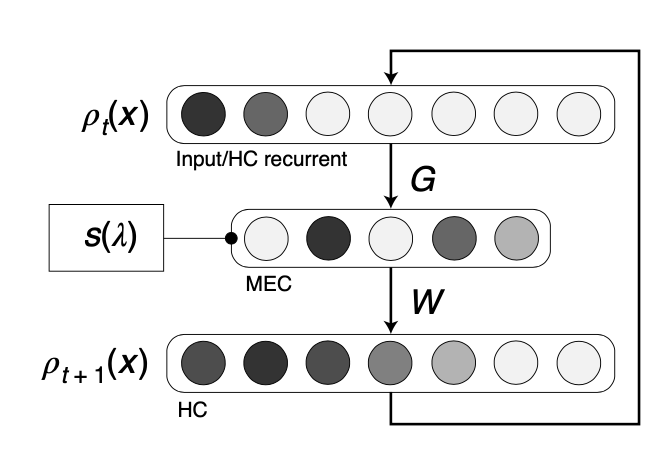
Considering the biological meaning of this genrator-based solution, sequence generation can be interpreted as a linear feedback loop of the EHC: current state profile is transformed to MEC via equating spectral components \(\phi_k\) (columns of \(G\)), rescaled by power spectrum \(s_{\tau}(\lambda)\), and readout to the hippocampal layer by \(W\).
To check biological plausibility of this model, D.C. McNamee, et al., 2021 checked firing maps for \(G\) matrix which optimizes the equation below for a random-walk generator \(O^{\text{rw}}\):
\[\text{argmin}_{G^{\top} G= I, G\geq 0} \left\| O-G\Lambda G^{\top} \right\|^2 _{F}\]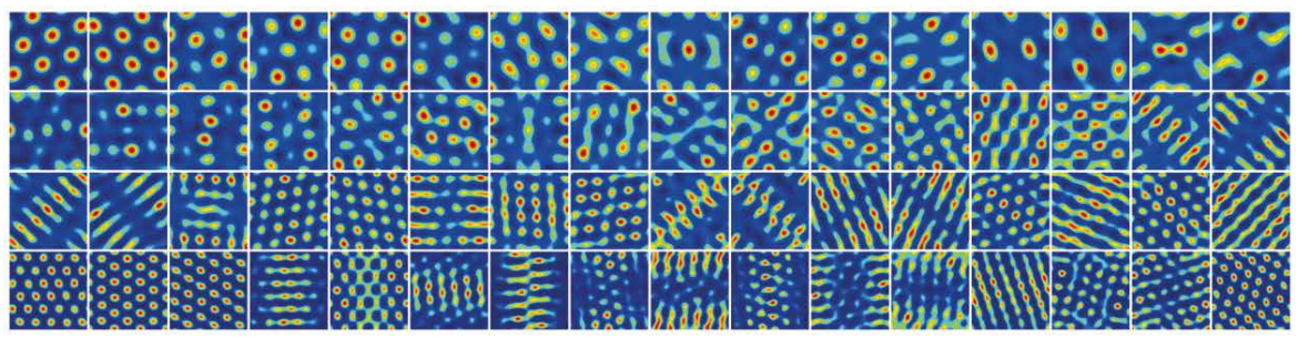
As a result, \(G\) matrix optimzed for a random-walk generator has shown hexagonal firing fields across multiple spatial scales.
Expanding sequence generation by Lévy flight hypothesis
Imagine a case where the rodent seeks for food. Without knowledge about where exactly the food may be located, the rodent must efficiently search through each location using its exploration process. In the aspect of computation theory, this problem can be restated as maximizing efficiency of random samply while maintaining low-complexity. If the rodent repeatedly samples target states at large spatial scales (\(\tau \rightarrow 0\)) then it will traverse the environment expending too much energy. In contrast, a small-scale search pattern (\(\tau \gg 0\)) will lead the rodent to oversample within a limited area, thus taking too long to fully explore the environment.
This conundrum has been extensively studied, which leads us to the Lévy flight foraging hypothesis. This hypothesis assumes animals tend to use Lévy flight strategy rather than simple Brownian motion when they seek for food, thus being forced to efficiently search through the field.
Then what is Lévy flight? Lévy flight is any random walk in which the step-lengths follow a Lévy distribution while the steps are in isotropic random directions. Due to its efficiency in search optimization, people who study biology started this walk strategy might also appear in animals as a consequence of natural selection. While whether this hypothesis holds to be true is controversial, it is quite interesting perspective to use this hypothesis in hippocampal sequence generation.
A general class of stable distributions known as symmetric Lévy \(\alpha\)-stable distributions, which includes Gaussian distribution as its special case, can be defined as below:
\[\varphi_{\alpha, \mu, c}(k) = e^{ik\mu -\left| ck \right|^{\alpha}}\]\(p_{\alpha, \mu, c} (x) = \frac{1}{2\pi} \int _{-\infty} ^{\infty} \varphi_{\alpha, \mu, c}(k) e^{-ikx} dk\) \(\mu\) parameter is zero in the random walk propagator since it is centered at the initial position, if we compare the above equation with our propagator equation \(P_{\tau} = G e^{\tau^{-1}\Lambda} W\), the scale parameter \(c\) turns out to be analogous to the parameter \(\tau\). Likewise, frequency \(k\) in the Fourier transofrm is equivalaent to the generator eigenvalues. As a conclusion we can say:
\[\mu \rightarrow 0\] \[c^{\alpha} \rightarrow \tau^{-1}\] \[k \rightarrow \lambda_k\]Then, the power spectrum matrix component can be re-written as
\[s_{\tau, \alpha}(\lambda) = e^{-\tau^{-1} \left| \lambda \right|^{\alpha}}\]which still includes the original case (\(\alpha=1\)). Remind that there is a negative sign added to the extended version of power spectrum due to the fact that \(\lambda \leq 0\).
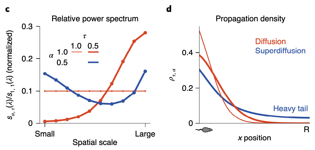
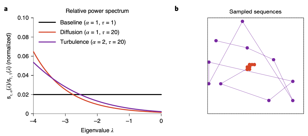
So since now we’ve got a more general version of the analytic solution of the state sequence generation, some of you might want to ask what exactly the role of \(\alpha\) is. As we can see in the above figure, although \(\alpha\) plays its role in balancing global and local search, how it influences balance between two scale search pattern is different with \(\tau\): by setting \(\alpha < 1\), both small and large scale spectral components are upweighted while the intermediate scale is suppressed. This non-monotonous power spectrum allows the agent to search in a large scale aspect, while keeping it’s attention in small scale searching as well. As a result, the propagation density when \(\alpha < 1\) follows a heavy tail distribution, also known as ‘superdiffusion’, allowing the propagator to have more ability to propagate to states distant from the current state.
We should however not underestimate \(\alpha\)’s power in sequence generation simply as giving the propagator the ability to search through large-scale. By modulating \(\alpha\), we can decide which spatiotemporal scale for the propagator to be sensitive to, leading to scale invariance.
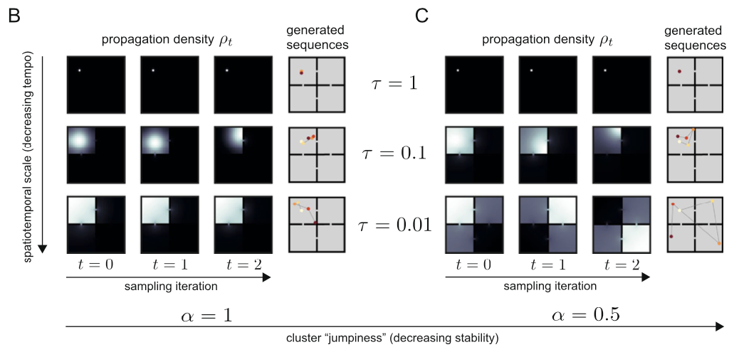
When \(\alpha = 1\), the generated sequence is quite stable for all cases of \(\tau\). If \(\alpha = 0.5\) however, when \(\tau\) is small enough, the sequence can ‘jump’ to different parts of the maze.
So I would like to say if \(\alpha < 1\), the propagator gains it’s abiility to sometimes jump to states which are quite distal (which would be states that are rarely visited when propated diffusively) from the current state.
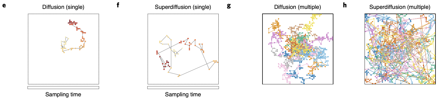
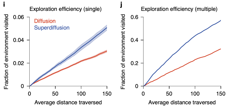
By comparing diffusivive sequence geneartion with superdiffusive case, we can easily see difference in spatial exploration efficiency: while supperdiffusive trajectories visit positions in an approximately homogeneous distribution across all areas, diffusive trajectories faiiled to fully explore all areas.
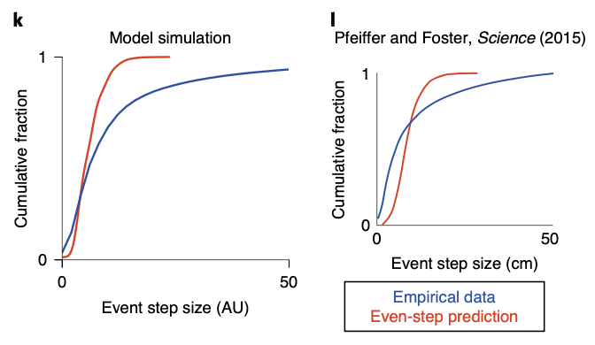
Interestingly, superdiffusion is not only superior to diffusion, but also more biologically plausible. B.E. Pfeiffer and D.J. Foster, 2015 have found that the cumulative fraction histogram of hippocampal sequence generation does not follow the expectation when assuming evenly spaced steps. This meant hippocampal sequence generation occurs in a spatially discontiguous form. As we can see in the figure below, this long-tail histogram can be reproduced in superdiffusive case, implying it’s biological plausibility.
The superdiffusive method explains another interesting phenomenon which was observed in B.E. Pfeiffer and D.J. Foster, Nature, 2013. When a rat recieves a reward repeatedly from a single spot while navigating an open arena, the rat can remember the reward location and engage in goal-directed navigation to acquire the reward. Interestingly, neurons in the dorsal hippocampal CA1 region over-represent the reward location not only when they are near the spot (home-events), but also when they are away from it (away-events).

This interesting phenomenon can be explained by the superdiffusion model. Let us define jump time \(J_i\) for a state \(x_i\) as the time interval from when a random process arrives at state \(x_i\) to when it leaves to another state. If we assume jump time \(J_i \sim \text{Exp} (\eta_i)\), jump rate \(\eta_i\) dtermine a temporal localization of state occupation, which would be:
\[P(J_i \leq \Delta t) = 1 - e^{- \eta_i \Delta t}\]where \(\Delta t\) is the time that process remains at \(x_i\) after arriving there. Thus, given that \(J_i\) scales as \(v_i J_i \sim \text{Exp}(v_i ^{-1} \eta_i)\) under \(v_i > 0\), decreasing the exponential parameter leads to an increase in expected jump time. Motivated by this idea, by scaling the generator transition rates at home states according to \(v^{-1}O_h\) where \(h\) indexes home state \(x_h \in \mathcal{X}\), we can control the remote activation of the rewarded home location.

When we generate sequence using the modulated propagator, the superdiffusive method succeed in resembling the over-representation of goal location even in away-events, while the diffusive method fails to. This result also indirectly supports the biological plausibility of superdiffusive model of hippocampal sequence generation.
D.C. McNamee, et al., 2021 has also shown impressive analysis in multi-goal foraging in a circular track environment, but I will skip this part in this blog post. Those who are interested in this are highly recommended to read the full paper.
Brain changing it’s mode in sequence generation
Majority of planning algorithms have evaluation of possible future trajectories as their critical element. To do so, many simulations use Monte Carlo Tree Search (MCTS). To evaluate the future trajectories, MCTS retrieve rewards associated to sampled state sequence. For example, the estimated reward \(\hat{r}\) of sampled states \((x_1, \cdots , x_N)\) will be
\[\mathbb{E}[r] \approx \hat{r} = \frac{1}{N} \sum _{i=1} ^N r(x_i)\]when \(r(x)\) is the reward function of state \(x\). If we sequentially sample states from a propagator, retrieving rewards and estimating the average reward using the equation above forms a Markov chain Monte Carlo (MCMC) algorithm. MCMC however may take a long time for a high quality of set of samples to be generated. This is because samples must be representative of the target distribution to ensure the Monte Carlo estimator is unbiased. To achieve samples to represent the whole target distribution, samples must be less correlated to each other.
This challenge in MCMC are undermined by the same issue, named generative autocorrelations in the Makov chain. First, the Markov chain can have initialization bias, meaning it did not forget where it started (thus has not converged). Second, even it cases where the chain has converged, successive samples might be strongly related, therefore providing limited amount of extra information independent of the previous.
To extract a set of samples that are decorrelated, we can mainly use two strategies:
1) Remove some of initial samples under the assumption that they are not drawn from a stationary distribution
2) Only accept samples generated at a period greater than 1
The quality of the MCMC estimator can be quantified by its sample variance \(\mathbb{V}_{\text{dyn}} \left[ \hat{r} \right]\). Let us assume a set of samples are independently drawn from \(x^{(i)} \sim p(x)\). The estimation uncertainty can be evaluated based on the sample variance of the estimator \(\hat{r}\):
\[\mathbb{V}_{\text{ind}}\left[ \hat{r} \right] = N^{-1} \mathbb{V}_p [r]\]where \(\mathbb{V}_p\) is the variance of the distribution \(p\). However, remind that it is impossible to directly generate independent samples from a stationary distribution since we do not have access to all possible state \(x \in \mathcal{X}\). Agents move around the state space to sample state sequences, forming a MCMC algorithm as we mentioned above. The sample variance \(\mathbb{V}_{\text{dyn}} \left[ \hat{r} \right]\) of a MCMC estimator is proportional to the integrated autoccorrelation time \(\Delta t_{ac}\):
\[\mathbb{V}_{\text{dyn}} = \Delta t_{ac} N^{-1} \mathbb{V}_p [r] = \Delta t_{ac} \mathbb{V}_{\text{ind}}\left[ \hat{r} \right]\]where
\[\Delta t_{ac} = \sum_{\Delta t = 0} ^{\infty} C_X (\Delta t)\]and \(C_X(\Delta t)\) is the autocorrelation function of the random state variable \(X\) at lag \(\Delta t\). We can see that the MCMC estimator’s sample variance \(\mathbb{V}_{\text{dyn}}\) achieves it’s minimum possible value when \(\Delta t_{ac} = 1\), since \(C_X(0) = 1\).
We can therefore intuitively interpret \(\Delta t_{ac}\) as the average number of iterations required to generate a single independent sample. This means the better estimation accuracy you desire, the longer sampling time is required. In MCMC estimation however, there exists a fundamentally different solution to solve this autocorrelation problem.
Let us define a binary one-hot random vector \(X\) such that \(X_i(t) = 1\) if and only if state \(x_i \in \mathcal{X}\) is sampled on time step \(t\). Otherwise, the value of \(X_j\), \(j \neq i\), is zero. Then the autocorrelation of \(X\) at lag \(\Delta t\) from initial time step 0 is the expectation
\[C_X (\Delta t) = \left< X(0) X(\Delta t) \right> = \left< \sum_{i=1} ^{\left| \mathcal{X} \right|} X_i(0) X_i(\Delta t)\right> = \sum_{i=1} ^{\left| \mathcal{X} \right|} \left< X_i(0) X_i(\Delta t)\right>\]Since \(X_i(0) X_i (\Delta t) = 1\) if and only if state \(x_i\) is sampled at time 0 and at lag \(\Delta t\),
\[\left< X_i(0) X_i(\Delta t)\right> = p(x=x_i, t=0)p(x=x_i, t=\Delta t | x=x_i, t=0)\]Using the spectral propagator we’ve derived in the previous section,
\[C_X (\Delta t) = \sum_{i=1} ^{|\mathcal{X}|} \rho_0(x_i) \left[ GS^{\Delta t} W \right]_{ii}\]where \(\rho_0 (x_i)\) is an intial distribution of states. Let us define a tensor \(\Gamma\) as
\[\Gamma_{kij} = \phi_k(x_i)\psi_{k}(x_j)\]where \(\phi_k\) is the \(k\)th column vector of \(G\) and \(\psi_k\) is the \(k\)th row vector of \(W\). Then the autocorrelation function can be expressed as
\[C_X(\Delta t) = \sum_{k=1}^{|\mathcal{X}|} \sum_{i=1}^{|\mathcal{X}|} \rho_0(x_i) \Gamma_{kii}s_{k}^{\Delta t}\]Now we can see that the autocorrelation function depends on the spectral power \(s\). By modulating the spectral power, we can minimize the autocorrelation between sequences. The spectrally-modulated propagator however are necessary to define a valid transition matrix, leading to it’s linear constratints as below:
\[\sum_{k=1} ^{|\mathcal{X}|} \Gamma_{kij}s_k \geq 0 \\ \sum_{j,k=1} ^{|\mathcal{X}|} \Gamma_{kij}s_k =1\]The first constraint ensures that all elements in the propagation matrix are positive, while the second constraint ensures the probability density to preserve under time evolution. The minimally autocorrelated power spectrum \(s_{\text{mac}}\) can be obtained using standard optimization routines.
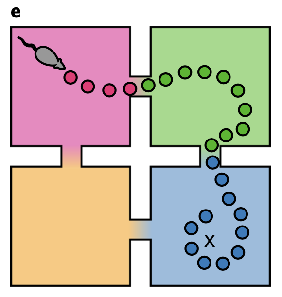
So when would it be useful to generate sequences using a propagator with minimally autocorrelated power spectrum \(s_{\text{mac}}\)? Since sequences generated using it would be highly decorrelated from each other, it has advantage in covering points where states can diverge according to the decision the agent makes. This hypothesis can be tested in a spatial alternation task where a rodent is required to make a binary decision at a junction, leading to a reward or nothing.
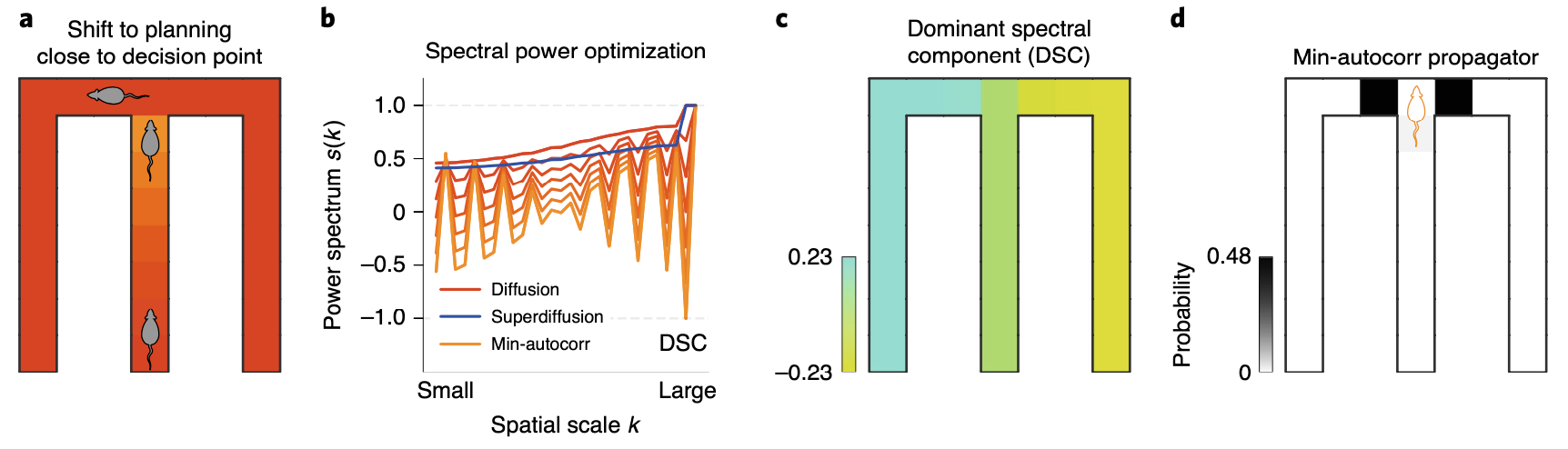
Based on our hypothesis, we can assume that the rodent would shift it’s planning based on minimally autocorrelated power spectrum near the decision point. If we compare the power spectrum between diffusion, superdiffusion and minimally autocorrelated propagator, the minimally autocorrelated case exhibit a significantly dissimilar profile.
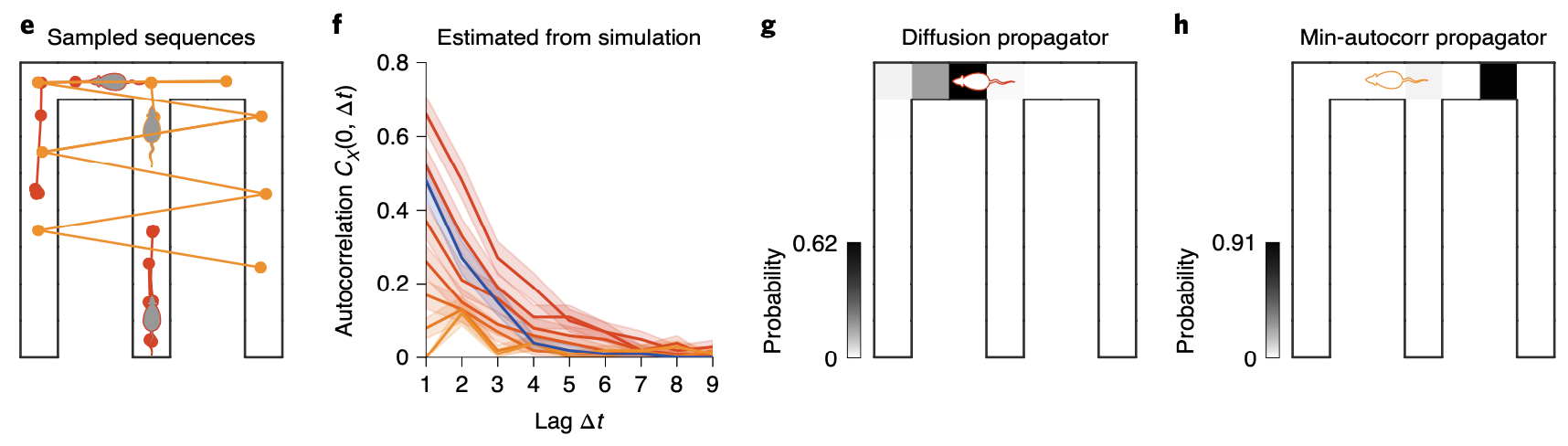
One interesting result is that the most inhibited spatial scale in \(s_{\text{mac}}(k)\), named as dominant spectral component (DSC), reflects a hierarchical deomposition of the state-space into three arms of the maze. Note that this spatial scale are actually over-weighted in both diffusion and superdiffusion. Then why would DSC be underweighted in minimally autocorrelated power spectrum? By inhibiting this spatial scale in it’s representation, the propagator is allowed to make sequences that can jump from one of the arm to the opposite side. Since it is very rare for an agent to reach a position on the counter side after entering one of the arms when it moves in a diffusive manner, these absurdly generated sequences seems satisfactory to make decorrelated sequences in MCMC. This interpretation is supported by the simulated results as below:
We have discussed three different types of sequence generation regimes in this post: diffusion, superdiffusion, and minimally autocorrelated. But how and when exactly these various types of sequence generation each occur? Spatial trajetories inferred by sharp-wave ripple (SWR) measured during rest period (sleep SWR) and active exploration period (wake SWR) in F. Stella et al., 2019 exhibit distinct stability modulation between sleep and wake periods. This distinct pattern can be explained simply by modulating \(\alpha\) value in the propagator model we’ve been discussing.

Rodents tend to use superdiffusion sequence generation during the exploration period, whereas they use diffusion sequence generation during the rest period. Recalling that memory consolidation mostly occurs during rest, we can presume diffusion sequence generation might play a role related to learning rather than decision making.

By comparing three sequence generation regimes while radomly walking on a ‘ring of cliques’ state-space, we can understand how these three regimes differ. Superdiffusion is optimized for exploration, while diffusion and minimally autocorrelated are optimized in learning and sampling-based estimation, respectively.
Hippocampus modeling in psychiatry, and questions remaining to be answered
It is exciting to mathematically understand the mechanism of hippocampal replay, and this knowledge might not only lead us one step closer to artificial general intelligence but also to better understand psychiatric disorders.
Patients with schizophrenia often fail in conceptual organization, which is reflected in positive symptoms such as delusions, hallucinations, and disorganized speech. Conceptual organization requires the ability to understand relational structure between nodes in the internal semantic space. Since understanding relational structure is one of the core ability required to generate ‘reasonable’ sequence as well, we can naively hypothesize that patients with schizophrenia might also show abnormal features while hippocampal replay.
Remind that we have only discussed the sequence generation reigme in case of \(\alpha \leq 1\). What happens when \(\alpha > 1\)? This is the case where we call the turbulent regime. In this case, the trajectory generated sample states in a random manner, thus being inconsistent with the spatiotemporal structure of the environment. (Bottom figure right, purple lines)
The spiking cross-correlation between place cells as a function of the distance between their place fields resemble a characteristic ‘V’ pattern, meaning the greater the distance becomes, place cell activate after larger time intervals. In a genetic mouse model of schizophrenia (forebrain specific calcineurin knockout mouse) however, lost this correlation pattern. This pattern can be reproduced via simulation by using diffusion and turbulent regime for sequence generation, respectively.

These results suggest at least some postivie symptoms shown in schizophrenia might be caused by turbulent sequence generation in the hippocampus, rather than other stable regimes. It is not surprising however to point out hippocampus as a candidate to explain the pathophysiology of schizophrenia. Patients with schizophrenia show cognitive impairment in a general manner, especially in working memory, processing speed, which are cognitive functions hippocampus plays a major role in.
It might be hard to directly use the hippocampal sequence generation model we’ve discussed in this post to unravel the mysterious pathophysiology of schizophrenia due to it’s complexity and limitations in obtaining high resolution neural signals from patients. The great power of computational model however is that we can derive interesting new hypothesis and design a clever experiment to confirm whether the hypothesis would be right or not. This would lead us to define symptoms of schizophrenia in a more objective language - mathematics, and develop diagnostic criteria which reflects the pathophysiology of the disease, rather than the symptom.
Although the paper we’ve discussed in this post is a great work by Matthew Botvinick and Sam Gershman (and their colleagues), some questions still remain as a msytery.
First, what is the biological substance of \(\alpha\)?
Second, how does the brain modulate which sequence generation regime they will use?
It is my pleasure and luck to see talented neuroscientists unraveling fundamental questions about intelligence. And as a wish, I hope there would be some space for me to be part of this exciting game.