
Despite the overwhelming victory of AlphaGo against human beings in 2016, artificial intelligence still does not replace human beings in many fields. Most artificial intelligence that has shown human-like (or even superior) performance in decision-making tasks is based on reinforcement learning algorithms. These algorithms however do not fully implement the ability to generalize what they have learned from millions of trials: if it is placed to another task, it will need another tremendous trial to learn to be good at it.
Animals in contrast have the flexibility to transfer knowledge learned from one domain to another. This enables them to quickly learn and adapt to new situations. People who study intelligence define this ability as a generalization. If an intelligent system has truly understood the structure of the task, it can simply use the knowledge to adapt to tasks with the same structure, but different stimuli. Making artificial intelligence understand the task structure is therefore the key to unlock the ability of generalization. Although it is not the only way to solve big questions in artificial intelligence, taking inspiration from the field of neuroscience is a very efficient approach to do so.
Hippocampus and Entorhinal cortex: Capturing task specific features
The hippocampus is known to play important roles in various kinds of cognitive processes including generalization, memory, one-shot imagination, and navigation. The well-known successor representation model suggests place cells and grid cells found in the hippocampus and entorhinal cortex emerge based on learning the state transition matrix. According to conventional reinforcement learning algorithms, we can define the state value function of state \(s\) as below:
\[V(s)=\mathbb{E} \left[ \sum_{t=0} ^{\infty} \gamma^t R(s_t) | s_0 = s \right]\]where \(s_t\) is the state visited at time \(t\), and \(\gamma \in [0, 1]\) is decaying discount factor. The idea of successor representation is to decompose the value function into the inner product of the reward function with predictive representation of the state (SR), denoted \(M\):
\[V(s) = \sum_{s'} M(s, s')R(s')\] \[\text{where } M(s,s') = \mathbb{E} \left[ \sum_{t=0} ^{\infty} \gamma^t \mathbb{I}(s_t = s') | s_0 = s \right] = \sum_{t=0}^{\infty} \gamma^t T^t\]where \(T\) is the transition probability matrix.
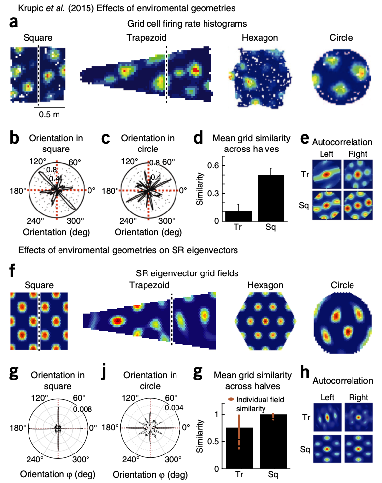
As shown in the figure (K.L. Stachenfeld et al., Nature Neurosciene, 2018) above, the grid cell firing rate histograms are highly alike the low-dimensional eigendecomposition of the successor representation. These results suggest that the entorhinal cortex captures important features of the task structure.
Much research implying the important role of the hippocampus and entorhinal cortex in understanding and representing the task and stimuli cemented a theory neuroscientists are highly interested in, called cognitive map theory. Unlike the traditional belief that the hippocampus and its nearby structures have a very unique pattern in representing spatial memories, studies have begun suggesting that these brain regions similarly represent non-spatial dimensions.
Hippocampal-entorhinal system in ANN
A study published by DeepMind (A. Banino, et al., Nature, 2018) showed emergence of grid-like representations in neural networks using supervised learning. Thus, it indirectly proved the efficiency of grid-pattern coding to represent states in a spatial navigation task.
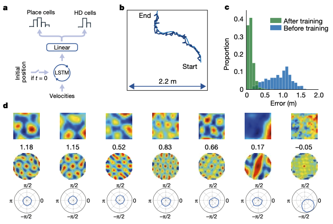
Still, the neural network required ground truth labels of what to predict: in this case, the actual \(x, y\) coordinates. Since \(x, y\) coordinates of the agent is the most crucial feature to represent current states in spatial navigation task, approach done in the paper has limitations in explaining how animals and humans find what features they should learn to predict from high-dimension stimuli.
A paper published in NeurIPS 2018 (J.C.R. Whittington, et al. NeurIPS Conference, 2018) came up with a solution with this problem. Here, they considered an agent to passively move through a 2D graph while observing a non-unique sensory stimulus on each vertex. All task environments share the same structure, while varying in stimuli distributions. The agent should learn abstract representations of the task structure to quickly adpat to environments with different stimuli.
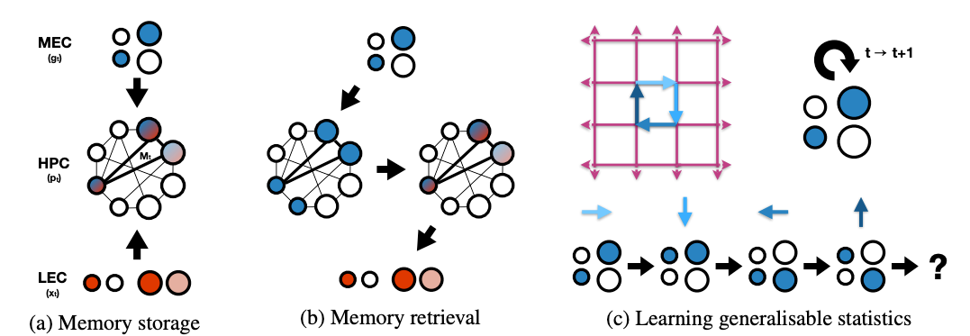
To acheive this goal, they propose grid cells to be the bases for constructing abstract representation of space, and place cell representation for the formation of fast episodic memories. Memories should link ‘what’ to ‘where’. In other words, memories need to conjuct location information with sensory stimuli. In this paper they suggest place cells to form conjunctive representation between the sensory input and grid input.
The model proposed in the paper has two different networks: Generative and Inference network.
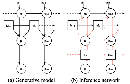
Generative Model
The agent have a generative model which factorises as
\[p_{\theta} (\mathbb{x}_{\leq T}, \mathbb{p}_{\leq T}, \mathbb{g}_{\leq T}) = \prod^T_{t=1}p_{\theta}(\mathbb{x}_t | \mathbb{p}_t)p_{\theta}(\mathbb{p}_t | M_{t-1}, \mathbb{g}_t)p_{\theta}(\mathbb{g}_t | \mathbb{g}_{t-1}, \mathbb{a}_t)\]where \(\mathbb{x}_t\) is the instantaneous sensory stimulus (one-hot vector where each of its \(n_s\) elements represent a sensory identity) and latent variable \(\mathbb{p}_t\) and \(\mathbb{g}_t\) are grid and place cells. \(M_t\) is the agent’s memory composed from past place cell representations, and \(a_t\) represents the current action. \(\theta\) are parameters of the generative model.
Inference Network
The posterior \(p(\mathbb{g}_t, \mathbb{p}_t \vert \mathbb{x}_{\leq T}, \mathbb{a}_{\leq T})\) is intractable, therefore we need to approximate it. The recognition distribution by the inference network can be factorised as below:
\[q_{\phi} \left( \mathbb{g}_{\leq T}, \mathbb{p}_{\leq T} \vert \mathbb{x}_{\leq T}\right) = \prod _{t=1} ^T q_{\phi}(\mathbb{g}_t \vert \mathbb{x}_{\leq t}, M_{t-1}, \mathbb{g}_{t-1}) q_{\phi}(\mathbb{p}_t \vert \mathbb{x}_{\leq t}, \mathbb{g}_t)\]where \(\phi\) denote the parameters of the inference network.
Grid Cells
Generative Model
From the equation above, \(p_{\theta}(\mathbb{g}_t \vert \mathbb{g}_{t-1}, \mathbb{a}_t)\) is a Gaussian transition probability density, with the transitions taking the form as below:
\[\mathbb{g}_t = f_{\mu_g}(\mathbb{g}_{t-1} + D_a \mathbb{g}_{t-1}) + \sigma \cdot \epsilon_t\] \[\epsilon_t \sim \mathcal{N}(0, \mathbb{I})\] \[\text{where } Vec[D_a] = f_D (\mathbb{a}_t), \,\, \sigma =f_{\sigma_g}(\mathbb{g}_{t-1})\]Some might struggle in understanding the exact meaning of \(D_a\). Remind that \(f_D\) is a multi-layer perceptron estimating the transition matrix for given action \(a_t\). Thus, \(D_a\) captures the state-to-state transition in the domain of \(\mathbb{g}\), which is the abstracted latent space to encode states. The paper mentions to give restrictions to connections in \(D_a\), so that connections are defined from low frequency to the same or higher frequency only.
Inference Model
\(q_{\phi}(\mathbb{g}_t \vert \mathbb{x}_{\leq t}, M_{t-1}, \mathbb{g}_{t-1})\) can be factorized as below:
\[q_{\phi}(\mathbb{g}_t \vert \mathbb{x}_{\leq t}, M_{t-1}, \mathbb{g}_{t-1})= q_{\phi} (\mathbb{g}_t \vert \mathbb{g}_{t-1}, \mathbb{a}_t) q_{\phi}(\mathbb{g}_t \vert \mathbb{x}_{\leq t}, M_{t-1})\]To know where we are, we infer grid code of current state \(\mathbb{g}_t\), and this can be successfully done by integrating the path, as well as using sensory information we have seen previously. Note that each approach is captured in the factorized term, respectively.
Place Cells
From the equation above, \(p_{\theta}(\mathbb{p}_t \vert M_{t-1}, \mathbb{g}_t)\) is a Gaussian probability density for retrieving memories. Memories of place cells are stored in Hebbian weights between place cells. The learning rule to update the memory is as below:
\[M_t = \lambda M_{t-1} + \eta (\mathbb{p}_t - \hat{\mathbb{p}}_t)(\mathbb{p}_t + \hat{\mathbb{p}}_t)^T\]where \(\hat{\mathbb{p}}_t\) represents place cells generated from inferred grid cells. So before we move on to details about how place cells store memories, let’s first go back and understand how they infer \(\mathbb{p}_t\).
As mentioned previously, memory is a conjunction between sensorium and structural information from grid cells. Sensorium is obtained by first compressing the sensory data \(\mathbb{x}_t\) to \(f_c(\mathbb{x}_t)\). This enables the sensory data \(\mathbb{x}_t\) to have same dimension as \(\mathbb{g}_t\). After so, it is filtered via exponential smoothing into different frequency bands, \(\mathbb{x}_t ^f\).
To clarify why they use exponential smoothing, let’s take a look at the definition of it. For time series \(x_t\), the simplest exponential smoothed value \(s_t\) will be:
\[s_0 = x_0\] \[s_t = \alpha x_t + (1-\alpha)s_{t-1}, \,\,\, t>0\]We can re-write this as
\[s_t = \alpha \sum_{k=0}^t (1-\alpha)^k x_{t-k}\]Now if we define \(\alpha x_{t-k}\) as \(c_k\) and estimate \((1-\alpha)^k\) to be \(\text{exp}(-k\alpha)\)
\[s_t = \sum_{k=0}^t c_k e^{-k\alpha} \approx \int_{0} ^{\infty} c_k e^{-sk} dk\]We can say exponential smoothing is actually Laplace transform when \(c_k\) is non-zero value only for \(k= 0 , 1, \cdots, t\). Thus, exponential smoothing with coefficient \(\alpha\) is very similar to Laplace transform of \(x_t\) with \(s=\alpha\).
Now coming back to the paper, exponential smoothing of \(\mathbb{x}_t\) can be considered as a simplified version of Laplace transform. By using different \(\alpha\) values, we temporally abstract \(\mathbb{x}_t\) in different time scale. (Imagine using real number exponential function instead of pure imaginary number in Fourier’s transform) Thus, exponential smoothing captures useful information in time domain, which is a well-known function of the lateral entorhinal cortex. After normalization step, each \(\mathbb{x}_t ^f\) is conjuncted with \(\mathbb{g}_t ^f\) to give mean of the distribution, \(q_{\phi} (\mathbb{p}_t \vert \mathbb{x}_{\leq t}, \mathbb{g}_t)\).
To retrieve memories, an attractor network of the form
\[\mathbb{h}_{\tau} = f_p (\alpha * \mathbb{h}_{\tau-1} + M_t \mathbb{h}_{\tau-1})\]is used, where \(\tau\) is the iteration of the attractor network and \(\alpha\) is the decay term. Depending on whether memories are being retrieved for generative or inference purposes, the input to the attractor, \(\mathbb{h}_0\), is from the grid cells or sensorium.
Tolman-Eichenbaum Machine
Using the model above, Timothy Behrens and his collegues recently showed that the model captures diverse properties that have been known to exist in real animal’s brain(J.C.R. Whittington, et al. Cell, 2020). They mention the model as ‘Tolman-Eichenbaum Machine’, since it reflects great ideas by Tolman and Eichenbaum.
The congnitive map theory was first proposed by Tolman at 1948, as he argued humans and other animals make complex inferences from sparse observations relying on a systematic ogranization of knowledge. Many neuroscientific researches showed that the hippocampus, especially during spatial tasks, has great contribution and reflect features of this mapping problem. On the other hand, hippocampus is also critical for non-spatial inferences that rely on understanding the relationships or associations between objectes and events. Although it has been a while since theory suggesting a common mechanism underlying both relational memory and spatial reasoning has been proposed, it remains unclear whether such mechansim exists or how it could account for the diverse array of apparently bespoke spatial cell types. Timothy and his collegues however, suggest the model they proposed in their 2018 NIPS paper might shed some light on answering this misterious question.
TEM can generalize structural knowledge
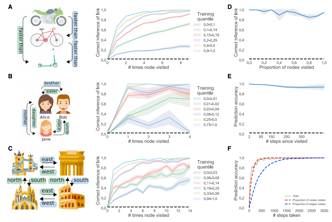
After training TEM, it was asked to make inferences in new transitive inference tasks without any additional experience. For example, after showing a sequence such as A>B>C>D>E, they are asked to answer “what is 3 more than E”, and has to answer as “B”. The same was checked for either social and spatial strucutral tasks, and TEM was able to answer correctly without having previously seen the particular sensory details of the task before as it has been exposed to similar relational structures. Thus, we can claim TEM acutally learns the structural knowledge, regardless of the particula sensory identities.
TEM represents structure with Grid Cells and forms memories with Place Cells
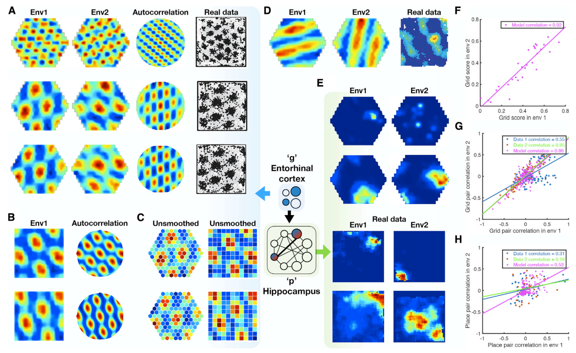
Surprisingly, when a TEM agent diffuse randomly on 2D graph, the learned \(\mathbb{g}\) representations resemble grid cells in both hexagonal space (A) and sqaure space (B). Not only does it resemble the grid like pattern, but it also learned gird-patterns with different frequencies and different phases. Learned memory reprsentations \(\mathbb{p}\), on the other hand, resemble place cells and have different field sizes. These cells remap between environments, which means they do not generalize.
By comparing real data with data from TEM, we can confirm that spatial correlation coefficients of pairs of TEM structural cells and real grid cells correlate strongly, while TEM hippocampal and real data place cells preserved their relationship to a lesser extent. In other words this means TEM structural cells (or real grid cells) encode more generalizable relationships than TEM hippocampal cells (or real place cells).
Entorhincal and Hippocampal Cell Types form a basis for transition statistics
As we discussed in the first section, we can interpret grid code as eigenvectors of the predictive representation of the state. The grid code pattern therefore, should soley depend on the transition matrix: in other words, for non-diffusive transitions, medial entorhinal representation must change its pattern resembling fundamental properties of it’s transitions. So does medial entorhinal representation \(\mathbb{g}\) in TEM reflect this phenomenon? The answer is yes.
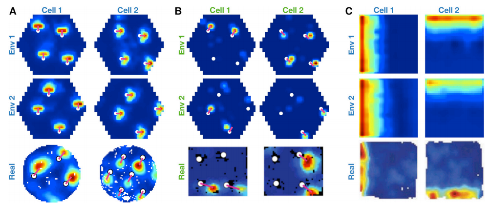
When non-diffusive transition is applied to the agent by mimicing behavior tendencies of animals to spend time near boundaries and aproach objects, the \(\mathbb{g}\) representations now shape into border cells (C) and object vector cells (A). The emergence of object vector cells is quite obvious. Since TEM learns predictive representations and the agent has strong tendency to spend time near objects, \(\mathbb{g}\) should predict the next transition to be towrd an object - which is exactly what object vector cells do.
Another important finding is that although the hippocampal code \(\mathbb{p}\) represent vector to particular objects, unlike the \(\mathbb{g}\) representation they do not generalize across objects. (B) This type of cells are ‘landmark cells’, which have been found in rodent hippocampus.
Structural knowledge is preserved over apparently random hippocampal remapping
Now you might have captured some feeling of the difference between \(\mathbb{g}\) representation and \(\mathbb{p}\) representation. While \(\mathbb{g}\) represent fundamental structural knowledge of the environment (thus representing generalizable features of the task structure), \(\mathbb{p}\) represent more specific features.
Remind that TEM is based on a critical assumption that hippocampal representations \(\mathbb{p}\) depend on \(\mathbb{g}\) representations. Since \(\mathbb{g}\) representations are periodic, hippocampal place cells simply need to retain their phases with respect to the grid code. If the agent faces a new environment, the hippocampal place cells will be able to remap while retaining structural knowledge because place cells might move to the same phase but with repsect to a different peak.
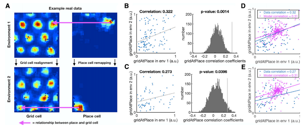
To confirm whether this explanation is biologically plausible, they tested data obtained from mouse and rats while they frrely foraged in multiple environments. If the place cell fires at the same grid phase in each environment, same grid cell will have strong activity at each place cell peak. Thus, by measuring the correlation of the activity of each grid cell at the peak firing of each place cell peak (gridAtPlace) across environments, we can check whether place cells after hippocampal remapping share the same grid cells with its predcecessor. The correlation across environment was statistically significant, supporting the hypothesis that place cells retian their relationship with the entorhinal grid, desptie remapping across environments.
Meachanistic understanding of complex non-spatial abstractions
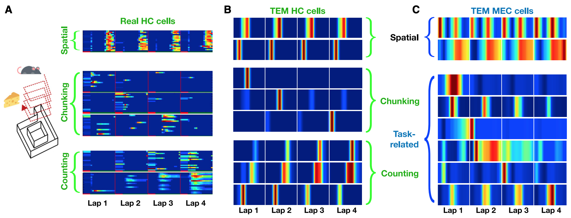
Since TEM’s objective function does not restrict itself to spatial tasks, TEM can learn arbitrary structural abstractions, including complex non-spatial tasks. In a recent study by Tonegawa and his collegeus (Sun et al. Nature Neuroscience, 2020), rodents perform laps of a circular track but only receive reward every four laps. Here, they found three different type of hippocampal cells: spatial place-cell like cells (A - top), cells preferentially firing on a given lap (A - middle), and those that count laps (A - bottom). When the TEM agent was given to learn the same task, all three types of hippocampal cells have emerged from it’s hippocampal units. (B)
What makes this experiment more interesting is that we can look into TEM’s medial entorhinal cortex cells to reveal a candidate mechanism of how animals learn these complex non-spatial features. As doing so, we can see that MEC cells learn both spatial and task-related non-spatial features. (C) Although these results stand only as a prediction since Sun et al., 2020 did not record MEC cells, the fact that MEC learned features are essential basis of hippocampal representations is indirectly proven: when the entorhinal cortex is manipulated, it disrupts lap sensitive hippocampal cells. Thus these results suggest that entorhinal cortex can learn to represent task structures in multiple level of cognitive abstractions simultaneously.
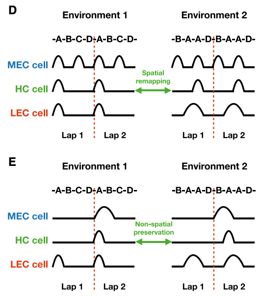
In non-spatial tasks, hippocampal cells remap to new spatial locations, but with preserved non-spatial lap specificity: they will preferentially fire on the same lap in each environment. To understand why this happens remind that hippocampal cells can only fire when both MEC and LEC cell fire together. Since non-spatial MEC cells (here, lap cells) encode number of laps rodents have made, hippocampal cells can fire only when the stimuli is given in the same lap.
Hippocampus and nearby structures as abstraction machines
All neuroscientists will agree that the hippocampus plays important role in memory and learning. What exactly and how our hippocampus learns however stayed a mystery for a long time. As proposed in several papers mentioned in this post, it is now believed that hippocampus and entorhinal cortex plays important role in finding useful representations of states in solving tasks. Considering how TEM is trained, we can conclude that the hippocampal-entorhinal system learns representations by predicting the next state. Learning domain knowledge by predicting the future outcome is one of the most well-known approaches in unsupervised learning (i.e. Oord et al., 2018), so it is not surprising that the brain uses a similar approach to learn state representations.
Recall K.L. Stachenfeld et al., 2018’s interpretation of grid cell patterns as an eigendecomposition of successor representation. This interpretation shares the predictive role of the hippocampal-entorhinal system with TEM. Combining ideas of these two approaches, I would carefully say the ‘grid frequency’ learned in TEM might be the eigenvalues of successor representations.
In this post, I have briefly summarized recent computational approaches explaining how the hippocampus contributes to inferring task structures and learns useful state representations. I believe by understanding the elegancy of the hippocampal-entorhinal system, we will find our way in reaching what we call artificial general intelligence (AGI).